Map Viewer Help

Map Viewer is a application for the creation, editing and analysis of maps, primarily in the field of mobile robotics, but not restricted to that domain. It is used for the creation, viewing and editing of vector maps and occupancy grids. It can load and save maps in a number of different formats, from many of the leading robot-simulation and control applications, such as CARMEN (http://www-2.cs.cmu.edu/~carmen/), Saphira (http://robots.activmedia.com), Player/Stage and BeeSoft, as well as having the ability to import/export images. Map Viewer can be used to edit maps, either by painting on them, or by drawing vectors on the map. It can translate between grid and vector maps, perform various statistical analysis functions on maps, average one or more maps, calculate Voronoi diagrams of maps and plan paths in a map, and randomly create new maps complete with obstacles, doors, rooms and corridors. Each of these features is discussed below.

1.01 History

The initial development of Map Viewer, up to version 1.6, stemmed from my masters in mobile robotics, the mouthful that is “An Empirical Evaluation Of Map Building Methodologies in Mobile Robotics Using The Feature Prediction Sonar Noise Filter And Metric Grid Map Benchmarking Suite”. The thesis is available on my website http://www.skynet.ie/~sos if you’d like to read it. I needed to be able to display maps for inclusion in my thesis, and also to perform some benchmarks. When I became interested in path planning, I decided to add some path planning functionality to the application. I also added a very basic (and very slow) Voronoi diagram generation algorithm, also for benchmarking purposes. The interface was ugly, the program was buggy as hell and seriously hungry in the memory stakes. However it was sufficient for my needs at the time, especially as I was the only one using it.

Cut to 6 months later, and I decided to teach myself to program an application with a proper user GUI in windows – most of my applications up to that point were of the command line variety, batch processing, parsers, compilers, AI routines etc. But I needed a project, so, in a fit of unoriginality I dusted off Map Viewer, came up with a project plan (which was thrown away and rewritten at least 50 times during development), and got going.

1.02 Reasons for developing Map Viewer

When looking for ideas of what could be included in the application, I first searched for anything similar to what I intended to write – an application to use in conjunction with mobile robotics to view and manipulate maps, either maps of the occupancy grid type (similar to a bitmap), or of the vector type (made up of lines). A few I found were CARMEN’s map editor, and Saphira’s map editor. There were a few other highly specialised editors also, each tailored to just a specific simulator. Both the CARMEN and Saphira editors are extremely basic, offering only very simple functionality, such as draw on occupancy grid (CARMEN) or place a line or rectangle on a map (Saphira). This is not to malign the rest of the software in these packages – both are extremely useful (I used Saphira for two years and all the results of my masters are based on my use of it), it just happens that their map editing software is probably each of their weakest points.

1.03 Primary Features of MapViewer

With the above in mind, I decided upon the following features to build in to Map Viewer version 2.0:

Make it compatible with as many robot simulators as possible, so as to widen the audience, but also to make work transferable from one platform to another.
Given the above, it must support both occupancy grids and vector maps, and the two should be interchangeable at runtime. Therefore it should be possible to load a Saphira vector map and save it as an occupancy grid for CARMEN or Player/Stage, and vice versa. Going from a vector map to a grid map was easy – going from a grid map to a vector map led to two separate line-fitting algorithms being developed. Also, any changes to a vector map should be reflected in the grid map.
Allow import/export of images, so scanned building plans can be quickly and easily converted into grid maps and vector maps.
Implement a layering engine to allow useful undo functionality, and also to allow vectors to be moved around the map, with the grid map being updated simultaneously.
Implement the full set of five benchmarks from my thesis. These measure the accuracy of a grid map against an ideal version of the map.
Implement a path planning functionality. This isn’t the most useful part of the application, but 90% of the code was already written, so I thought what the hell.
Create an easy to use, intuitive GUI for the manipulation of both grid maps and vector maps.
Enable the application to load a very simple grid map file format (described later) so any programmer can output their results and load it into Map Viewer. This is in contrast to applications like CARMEN and Player/Stage that use a relatively complex file format. This format can also, with a little editing of the file, be used in conjunction with gnuplot to display as a graph, if you should so wish.

MapViewer 2.0 was released in September 2004. I then began working on version 2.1. In addition to many, many minor bug fixes, the further additions included:

Build a grid map from sonar and odometry data. The algorithms used are detailed in my masters, mentioned above.
Add export support for the Rossum simulator. The Rossum simulator uses a vector-based map, similar to Saphira.

MapViewer 2.1 was released in October 2004. After feedback from some Player/Stage users, it became quickly apparent that the support for Player/Stage was far from perfect. This was down both to assumptions I made as well as the fact that Stage is extremely picky about what type of files it will load. Therefore, Player/Stage support was improved quite a bit, as well as a better redo functionality for MapViewer 2.12.

MapViewer 2.2 was released in January 2005, and included, in addition to some bug fixes, including a fairly major one with saving Saphira maps:

Randomly generate any number of maps, each containing any number of rooms and obstacles (memory permitting). This can be very useful for people who need to test their robots in a large number of statistically similar (or different) environments, and do not have the time to hand-craft hundreds of maps.

2. Types of maps used

Map Viewer deals with two different types of maps.

· Occupancy Grid - This represents area as a grid of equally sized squares, or cells. Each cell contains a floating point value between 0 and 1 inclusive, representing the probability that it is occupied. The higher the value, the more likely that there is an obstacle there. A value of –1 means that the cell in the map has not been altered. Many map building algorithms use this type of map (see papers by Moravec, Elfes, Konelige, Thrun, Fox, Burgard etc).

· Vector Map - This represents obstacles as straight line segments such as lines and rectangles. This type of map is useful to robot simulators as they are relatively simple to design and use few CPU or memory resources when computing a robot's interaction with them. Map Viewer supports four types of vectors

· Line – a simple straight line, one pixel wide

· Poly-line – a series of straight lines where consecutive lines begin where the previous

· Rectangle – a rectangle with sides one pixel thick.

· Filled Rectangle – a rectangle that is filled with a colour, or probability value. Not technically a vector, I know, and not (currently) supported by some simulators, e.g. Saphira.

Users can edit one or both map types simultaneously, and they are pretty much interchangeable. If you don’t care about Occupancy Grids, and just want to draw a vector map, you can. However, if vectors are drawn on the screen and the Occupancy Grid is visible, the vectors will automatically be integrated into the grid. This also goes for when they are deleted or moved – the grid will be updated accordingly. If this is not required, set the Occupancy Grid to non-viewable, and this processing/memory overhead will not occur.

It is also possible to place any number of robots on the map. Robots are circular with a line from the center to the circumference to indicate the direction they are facing.

3. File Menu

3.01 New Map

Creates a new map. Pops up a dialog requesting the width and height of the map, in millimetres. The default resolution of the map is 100, meaning that each pixel of the grid map represents 100mm * 100mm of the real world. This can be changed in the Edit menu.

3.02 Load Map Viewer Map

Loads either an occupancy grid, or a vector map, or both, from a file with the extension .mvm. This file type is specific to the map viewer application, and stores work-in-progress maps. At some point it should be saved as a format of some robot simulator or image.

3.03 Load Grid Map

Loads an occupancy grid. This can be in a number of different formats, including Carmen, BeeSoft, Saphira Laser Map, among others.

3.04 Load Carmen Grid Map

Loads a Grid Map in the Carmen format, which is documented on the Carmen website http://www-2.cs.cmu.edu/~carmen/ . Note that all information in the Carmen file not related to the grid map is discarded.

3.05 Load BeeSoft Grid Map

Loads a grid map in the BeeSoft format.

3.06 Load Stage World

Loads a world in the Player/Stage format – http://playerstage.sourceforge.net . This comprises of two files. The first, and the one you choose, is a text file with the extension “.world”. This describes the objects in the world, such as the robots. The second is an image file, usually with the extension “.pnm” or “.pgm”. This image is analogous to a grid map, and describes the position of obstacles in the environment.

3.07 Load Grid Map As List Of Points

Loads a grid map from a very simplistic grid file format. It starts with the word “gridpointlist”, followed by the width and height of the map. Then each point in the map is listed with its x position, y position and value of between 0 and 1. It looks like the following:

gridpointlist

width 100

height 100

xPos yPos cellValue

3.08 Load Saphira Wld Map

Loads a vector map in the Saphira (http://robots.activmedia.com) format. The Saphira format supports lines only, no filled objects.

3.09 Load Image

Imports an image file and converts it into a map. Current supported image types for import are JPEG, BMP and PNM (for Player/Stage grid maps). All images are converted on a 1 pixel to 1 grid cell basis. Each pixel is normalised to a value between 0 and 1 depending on it’s brightness, which means all images are converted to greyscale.

3.10 Load Path

Load a previously created path from a file with the extension .pat. For this to be meaningful, the path should have been generated on a map of the same environment it is being displayed on. The format of a path file is quite simple. The first entry in the file is the word “path”. As there can be multiple paths in a single file, each separate path is delimited by the words “begin” and “end”. Between these delimiters are the waypoints on the path in Cartesian coordinates, which break it up into straight line segments. A example of a path file is as follows, with two paths in the file, the first with two waypoints, and the second with three waypoints.

path

begin 118 40 312 43 end

begin 366 42 301 50 297 85 end

3.11 Load Path Goals

Loading path goal points (with extension .gol) loads the start and end points of a path and attempts to plot a path between those points with a modified A-Star algorithm. This differs from the Load Path menu item, which does not check if the path is valid. Upon loading the path goals, a dialog informs you how many paths were successful, and how many were not. The format of a path goal file is quite simple. It begins with the word “pathgoals”, then each start/end pair is represented by four numbers making up two Cartesian coordinates. For example, a path goal file with two paths looks like this:

pathgoals

118 40 312 43

366 42 297 85

The first path goes from the point (118,40) to (312,43), and the second from (366,42) to (297,85).

3.12 Load Voronoi Diagram

Loads a previously generated Voronoi diagram. A Voronoi diagram is a graph which represents the equidistant points between obstacles in a map. For a detailed discussion, there are a number of resources on the web – probably the best is www.voronoi.com. Also, the website of the author, www.skynet.ie/~sos, contains a masters thesis that discusses the uses of Voronoi diagrams when analysing maps, and explains the benchmark methods that can be applied to maps with Map Viewer. It also provides the code used to generate Voronoi diagrams for this application.

The format of a Voronoi file: it begins with the word “voronoi”. There are then three sections. The first starts with the word “lines”, and contains couples of Cartesian coordinates represented using floating point numbers. Each couple represents one straight line of the graph to be displayed, and may not be a complete edge, since an edge can be a curve and may therefore consist of many small straight lines. For example, a Voronoi file with three edges would look like this:

voronoi

lines

88.5 0 88.5 15.5

259.794 0 259.794 0

423.818 0 423.818 0

The second section begins with the word “edges”, and contains a list of all the edges in the graph. These are stored as vertex pairs. This information is used in the Voronoi-based benchmarks in Map Viewer.

The third section begins with the word “vertices”, and contains a list of all the vertices in the graph, which are the points where edges end. This is for display purposes, to show the joins in the graph.

3.13 Save Grid Map

Save the current grid map in Map Viewer’s own “.mvm” (Map Viewer Map) format. This will include all grid information, as well as all the vectors that have been added to the grid. While the vectors themselves will not be preserved, their grid-representation will be. Therefore, when this file is reloaded, it will not be possible to move the vectors around, rotate them etc, as they will only be represented as pixels.

3.14 Save Vector Map

Save just the vectors in the map (the lines, rectangles, filled rectangles and robots) in MapViewer’s “.mvm” format. No Grid (or pixel) information will be stored.

3.15 Save Vectors and Grid Map

Saves all information in MapViewer’s “.mvm” format. All pixel and vector information will be preserved. If this file is reloaded, it will be exactly the same as when it was saved.

3.16 Save Grid Map In Carmen Format

Save the current grid map in Carmen format, suitable for use with the Carmen robotic suite. This will include all grid information, as well as all the vectors that have been added to the grid. While the vectors themselves will not be preserved, their grid-representation will be.

3.17 Save Grid Map In BeeSoft Format

Save the current grid map in BeeSoft format. All vector information is lost, only grid (pixel) information is retained.

3.18 Save Grid Map In Stage Format

Save the current map in Player/Stage format. This saves two files. The first is a WORLD file, with the extension “.world”. This contains information about the placement of objects in the world, such as robots. The second in a PNM image file, which just stores pixel information. Therefore, all vector information is discarded, except for robots, which are stored in the WORLD file.

3.19 Save Grid Map As List Of Points

Saves the grid map as a list of points. This discards all vector information. This is a very simplistic grid file format, and is quite useful for exporting maps from map viewer into an easily understood format.

It starts with the word “gridpointlist”, followed by the width and height of the map. Then each point in the map is listed with its x position, y position and value of between 0 and 1. It looks like the following:

gridpointlist

width 100

height 100

xPos yPos cellValue

3.20 Save Vector Map As Saphira Wld

Save the vector map as a Saphira World file, with the extension .wld. Only vectors will be saved. No grid/occupancy information is saved. This file is for use with the Saphira robotic suite from ActivMedia (http://robots.activmedia.com).

3.21 Save Vector Map As Rossum Floor Plan

Save the vector map as a Rossum floor plan. (http://rossum.sourceforge.net ) . All pixel information is discarded, as the Rossum simulator doesn’t support it. All vectors and robots are written to the file.

3.22 Save as Image

Saves what is currently displayed as either a bitmap or a jpeg image. If a Voronoi diagram, path, vector and/or GridMap are displayed, it will all appear in the final image. There are two options when saving an image:

Save Complete Map – this saves the whole map, on a one cell to one pixel basis.
Save Current Zoomed Selection – Saves exactly what is currently on the screen, generally not in a one cell to one pixel basis.

3.23 Save Path

Saves all the paths currently in the application in a file with the extension .pat using the format described earlier.

3.24 Save Path Goals

Saves the start and end points of all paths currently in the application in a file with the extension .gol, using the format described earlier.

3.25 Save Voronoi Diagram

Saves the Voronoi diagram in a file with the extension .vor using the format described earlier.

4. Edit Menu

4.1 Undo

Undoes the last action. Up to 10 undo’s are possible.

4.2 Redo

Redoes the last undone action.

4.3 Set Resolution

Sets the resolution of the map – that is, the width (or height) of a single cell in millimetres. This only matters when saving a vector map in Saphira .wld format, or saving a CARMEN grid map.

4.4 Crop/Expand Map To Selection

Changes the size of the map to whatever the currently zoomed area is. If you are zoomed out more than the standard map size, then the canvas will get bigger. If you are zoomed in, then the canvas will become smaller. As well as the grid map being changed, all vectors are clipped to fit in the new area (if the new area is smaller than the old).

4.5 Translate Map

Translate the map in the X and Y directions.

5. View Menu

Each of the selections on the top area of this menu change whether or not a particular object is visible. These include the toolbar, status bar, ruler around the map, robots, robot runs, the Voronoi edges, the Voronoi vertices, the paths and the background grid that appears when viewing just the vector map.

The three bottom options, “Show Average/Min/Max Cell Value” change how a grid map is viewed. These only affect a grid map that cannot fit on the screen on a 1-pixel to 1-grid cell basis. This can happen either with a very large map or when zoomed out quite far. In this case, multiple cells are displayed in one pixel. The pixel colour can be an average of all cells in it (the default setting, and the one that most accurately condenses the map to fit the screen). The pixel can be the maximum value of all cells in it – this can be useful with very large, very sparse maps, with very few cells of non-zero values. The pixel can also display the minimum of all cell values – I don’t know what use this has, but it doesn’t hurt being in there.

6. Tools Menu

6.1 Convert Grid Map To Vector Map With Box Fitting

This takes a grid map and converts it to a vector map with a relatively simple algorithm called Box Fitting. It draws a rectangle around each grid cell above the user-defined threshold value, and joins together neighbouring rectangles. This algorithm is very lightweight and very fast – it runs in O(n) time. Using this tool, you can quickly create a vector map by ‘painting’ on the map grid, and then convert the grid to a vector map. It is also useful when existing grid maps are available, and you’d like to use them in a simulator that only supports vector maps.

This box fitting method does not give any information about groupings of cells, such as what general direction the cells are facing. That is done by the second conversion algorithm, Line Fitting.

6.2 Convert Grid Map To Vector Map With Line Fitting Using Cell Value

This takes a grid map and converts it to a vector map with an algorithm based on a combination of the sweep line Voronoi algorithm by Stephen Fortune and a grid map conversion algorithm developed for Map Viewer. It creates more realistic maps than the Box Fitting algorithm, since it fits lines to groupings of grid cells. In this way the direction that a group of cells is facing is determined. This is a more expensive algorithm than Box Fitting, and runs in O(nlogn) time. The “Using Cell Value” refers to the filtering applied to the grid before the line fitting takes place. All cells within a certain value range (e.g. between 0.5 and 1.0) will have lines fitted to them.

6.3 Convert Grid Map To Vector Map With Line Fitting Using Contrast

This is very similar to the previous tool, however the filtering applied to the grid before line fitting is different. In this case, the grid cells that will have lines fitted to them are chosen based on their relative value compared to the cells around them. Once the user has chosen a value (e.g. 0.3), then any cell that has an adjacent cell with a value more than 0.3 different from it will have a line fitted to it.

6.3 Average Grid Map With Another Grid Map

Averages the currently loaded grid map with another grid map. For example, if cell (100,100) in the currently loaded map has a value of 1.0, and a value of 0.5 in the other map you choose, the resulting map will have a value of 0.75 in the cell (100,100). Note that if you average a number of maps, a cumulative average is taken, so for example if a third map has the value of 0 in cell (100,100), the new value will be (1.0 + 0.5 + 0.0)/3 = 0.5. Also note that maps are averaged on a cell by cell basis, so they will have to be within the same coordinates.

6.4 Grid Map Benchmarks

A suite of five benchmarks for comparing the accuracy or similarity of grid maps is provided. A full and detailed description of all five are given in Chapter 5 of my thesis at http://www.skynet.ie/~sos .

6.4.1 Correlation

This is a statistical measure of similarity between maps that compares them on a cell-by cell basis, and also taking the standard deviation from the mean into account. Gives a result between 0 and 1, the higher the result the more similar the maps are. For more information, see Chapter 5 of the authors thesis at http://www.skynet.ie/~sos, or the papers “Developing a Benchmarking Framework for Map Building Paradigms” by JJ Collins, Shane O’Sullivan et al, and “A Quantitive evaluation of sonar models and mathematical update methods for Map Building with mobile robots” by Shane O’Sullivan et al, also available at that address.

6.4.2 Compare Grid Map With Another Map Using Map Score

Another method for statistically comparing two maps on a cell-by-cell basis. Gives a positive result representing the difference between the two maps compared. The higher the score, the more different the maps. A score of 0 means that the maps are identical. The score is not normalised to any value, and is based on a metric put forward by Martin & Moravec. For more information, see the sources mentioned above.

6.4.3 Compare Grid Map With Another Map Using Map Score Occ Cells Only

Similar to the standard Map Score technique, which compares all of both maps with each other. This method only compares how much the two maps’ occupied cells match up. See the documentation above for more information.

6.4.4 Path Comparison Benchmarks

The final two benchmarks, false positive and false negative path statistics, do not compare a grid map against another grid map. Instead, they compare a grid map against a Voronoi diagram.

The idea with the false positive path statistic is that you generate a Voronoi diagram in a map that you have generated with some map building algorithm. Then load an ideal version of that map (either manually drawn or taken from architectural drawings), load the Voronoi diagram and run the benchmark. It will then tell you how many of the paths in the sensor-generated map are invalid, and therefore how useful the generated map is to a robot.

The false negative path statistic is the opposite. For this, you generate a Voronoi diagram in the ideal version of an environment, then load in a sensor-generated version of the map, load the ideal-map’s Voronoi diagram and run the benchmark. It will tell you how many of the paths in the Voronoi diagram could be completed and how many could not. This tells you how much the mapping algorithm you used over-estimated the occupancy value of cells in the grid.

Note that all of these benchmarks assume that you already have a very good localistion routine running when the readings are being taken. The less accurate you odometry (or your estimation of where the robot it) then the less useful the benchmarks.

6.5 Generate Simple Configuration Space

This generates a configuration space of a user-defined dimension in the grid map. A configuration space defines the area in a map that a robot can actually travel in this. It is essentially a fancy name for taking each occupied grid cell and drawing other occupied grid cells around it out to a user-define radius.

6.6 Reduce Map To Values 0 and 1

This takes a threshold value from the user, and sets all values in the grid map below that threshold to 0 and all others to 1.

6.7 Smooth Grid Map

This takes a upper and lower threshold from the user. For each cell in the grid map that is between those two thresholds, if it is surrounded by three or more cells not within the thresholds, it is set to the average value of those surrounding cells. This can be used to clean up grid maps that have a lot of little dots speckled around them.

6.8 Translate Map

This translates the map in the X and Y directions.

7 Create Map

7.1 New Blank Map

Creates a new map. Same as the “File/New Map” command.

7.2 Build Map From Sonar Data

This takes a file with positional and sonar sensor data from a robot and builds a grid map from it. The format is as follows (all measurements are in mm). At the top of the file is information on the layout of the sensors on the robot – that is their distance from the center of the robot in (x,y) coordinates and the angle at which each one is facing. The bulk of the file is generally made up of sensor data. Each line of sensor data contains the (x,y,angle) of the robot in its first three positions, then the range readings of each of the sonars. Here is a short example file of a robot with seven sonars and a radius of 220mm.

robotrun

numsonars 7

start sonar

100 100 90

120 80 30

130 40 15

130 0 0

130 -40 -15

120 -80 -30

100 -100 -90

end

DATA SONAR

0 0 0 745 1047 757 762 725 1278 1043

1 1 5 1047 757 762 725 1278 1015

2 3 10 789 964 728 762 725 1278 1015

The first entry must be the word “robotrun”, then state how many sonars they are, then precede the list of sonar positions and angles with the terms “start” and “sonar”. The first entry, 100 100 90, specifies that the first sonar is at position (100,100) from the center of the robot, and is at 90 to the angle that the robot is facing. The robot is assumed to be facing to the right (i.e. along the x axis), which is angle 0. The state that the list of sonar positions are finished, use the term “end”.

As stated earlier, the bulk of the file will be the sensor data, of which just three records are shown here. The first three numbers on each line are the x, y and angle of the robot. The next seven numbers (it must be seven because “numsonars” was 7) are the ranges that each sonar measured. See the example files that come with MapViewer (they end in .run) for more examples.

7.3 Generate Random Map(s)

MapViewer has the ability to randomly generate any number of maps. Each map can have any number of rooms, and each room can contain a number of different obstacle types.

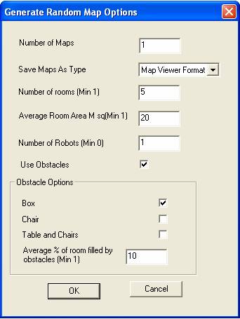
These are the following options:

· Number of Maps. If the default of 1 is used, the map is generated, and appears in the window. If more than one map is chosen to be generated, they must be saved to a file. A “Save Map” dialogue pops up to get the file name and path. All the files will be saved with ascending numbers appended to the end. For example, if you choose to save 3 maps in the MapViewer format, in the file “c:\maps\randomMap.mvm”, the files “randomMap1.mvm”, “randomMap2.mvm” and “randomMap3.mvm” will be created in the “c:\maps” directory.

· Save Maps As Type. This decides what format to save the generated maps in. It only matters if more than one map is generated.

· Number of rooms. Specifies the number of rooms in the environment. The environment is comprised of a number of rooms, interconnected by corridors.

· Average Room Area. Specifies the average area of all rooms. Each room will be a different width and height, but their area will average the number given here. The measurement is in Metres.

· Number of Robots. Specifies the number of robots to place in the environment. The robots will be placed in random positions in rooms chosen randomly.

· Use Obstacles. If this is checked, then obstacles will be placed in the rooms. There are three types of obstacles available.

Box. This is a simple rectangle, and can represent a vague obstacle.
Chair. A chair is a cross-shaped obstacle, which represents the base of a standard office-like wheeled-chair.
Table and Chairs. This is a table object surrounded on all sides by chairs. The table is rectangle in shape, with legs at the corners.

The number of each type of obstacle is weighted. For each table, there are two chairs and four boxes.

· Average % of Room Filled By Obstacles. This is used to determine how crowded the rooms are with obstacles. The smaller this number, the fewer obstacles will be in the rooms on average.

8. Extra Objects

This menu contains the objects that can be placed in a map, even though they’re not really obstacles like the lines and rectangles.

Currently, there are only robots in here. Click “Add Robot” to add a robot to the map, then click on the map to place the robot.

9. Clear Menu

Each of the options in this menu deletes an object, either a Voronoi diagram, all the paths, all the vectors, the grid map, or everything.

10. GUI Tools

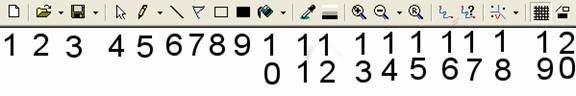
1. New Map – deletes everything and creates a new map.

2. Open Map, Image, Path or Voronoi diagram.

3. Save Map, Image, Path or Voronoi Diagram.

4. Select Vector – either click on a single vector to select it or draw a rectangle around a group of vectors to manipulate. When a vector is selected, it shows a number of handles, each of which allows you to either move or resize it.

5. Pencil – draws on the grid map with the current colour. You can select a various number of different pencil sizes with the drop-down menu.

6. Draw line.

7. Draw Poly-Line. Each line begins where the last one ended. To stop drawing, click the right mouse button.

8. Draw unfilled rectangle.

9. Draw filled rectangle.

10. Fill Tool. Fill an area of the grid map with the current chosen value. The drop down menu allows you to choose a tolerance level for the fill, i.e. how close to the clicked-on cell value do the other cells have to be to have their values changed.

11. Dropper Tool. Click on the grid map to choose the value of the clicked-on cell.

12. Colour Picker. Displays a dialog from which you can choose a value to use for the pencil and vector tools.

13. Zoom In. Draw a rectangle on the window to zoom in to that area.

14. Zoom Out. Clicking once zooms out 10%. The drop down menu allows you to choose different amounts to zoom out.

15. Reset Zoom. This fits the map to the window.

16. Create Path. Click on one part of the map to choose a starting point for a path. Click again to choose the end point. The first time you do this it may be a little slow, but afterwards it should be quite quick.

17. Path Options. Gives some options of how a path should be calculated. This is done with a series of weights as well as some other options.

18. Create Voronoi Diagram. This creates a Voronoi diagram in the current grid map. The drop down menu allows you to select how far apart two cells must be before a Voronoi edge will be plotted between them. If this value is less than the width of one cell (the resolution) then the Voronoi diagram will place a graph edge between every cell, making it essentially useless. Therefore, keep the value greater than the width of one cell.

19. View Grid Map. Displays and hides the grid map.

20. View Vector Map. Displays and hides the vector map.

11. Known Issues

The two benchmarks for path analysis are very memory hungry, and slightly buggy. This will be fixed in later releases.

12. Future Work

1. Animate the robot runs – instead of just showing the final path that multiple robots took, time splice and animate it.

2. Animate the creation of paths. This will show exactly how a path planning algorithm searched an environment in real time, instead of simply showing the final path. This can be useful when developing a new path planning algorithm. Users will be able to write out to a file in a given format the cells of the map that their algorithm processed in the order in which they were processed, and this can be animated with Map Viewer.

3. Support CAD file formats, to enable import/export to and from CAD packages such as AutoCAD.